CONTENTS
Production Volume and Reserve Growth vs. Profitability
Entry of Major Oil Companies Into Shale Plays
Evaluation of Shale Gas Well Performance
Well Performance Evaluation Methodology
Barnett Well Performance
Fayetteville Well Performance
Haynesville Well Performance
Comparison to Operator Claims
Matching Aggregate Production Profiles for Shale Gas Plays
Economics
Summary and Conclusions
Appendix
Production Volume and Reserve Growth vs. Profitability
Analysts, government agencies, academics and media pundits commonly equate large shale gas resource levels, production and reserve growth with commercial success. We do not dispute the impressive growth of shale gas resources, reserves or production. Examination of the balance sheets of the leading companies involved in shale gas development, however, reveals limited earnings or profit. We must ask the proponents of shale gas success to explain this fundamental discrepancy.
Some argue that price explains poor business results. First of all, whose fault is it that gas was over-produced to the point that prices were depressed other than the same companies that analysts praise for the shale gas revolution? Secondly, realized prices (the prices that results from hedging production volumes in advance of sales) over the past 5 or so years have never been higher because of high spot prices through mid-2008 and favorable hedge positions for much of the following period. This means that low prices cannot be blamed for lack of business success. The simple truth is that shale gas ventures are costly and profits are marginal at best.
Three decades of natural gas extraction from tight sandstone and coal-bed methane show that profits are marginal in low permeability reservoirs. Shale reservoirs have orders of magnitude lower reservoir permeability than tight sandstone and coal-bed methane. So why do smart analysts blindly accept that commercial results in shale plays should be different? The simple answer is found in high initial production rates. Unfortunately, these high initial rates are made up for by shorter lifespan wells and additional costs associated with well re-stimulation. Those who expect the long-term unit cost of shale gas to be less than that of other unconventional gas resources will be disappointed.
Entry of Major Oil Companies Into Shale Plays
Another common theme among shale advocates is that the entry of major oil companies into some of these plays proves that they are commercially viable. There are as many reasons for big companies to enter shale gas plays as there are big companies but the most obvious reason is reserves.
Reserve replacement has been a challenge for major oil companies for at least the last decade as opportunities in the international arena have contracted. North American shale gas plays offer a temporary solution. Whether big companies can find operational and technological ways to make these plays commercial is another question but, for the short term, shale plays provide a means to add reserves.
The notion that investment by large companies proves commercial success is disproved by recent history. We have to look no further than corn ethanol and other biofuel companies where optimistic claims of profitability are now seen to be unfounded. This is even with government mandated use, major subsidies, and import tariffs to protect domestic producers from competition. An excellent discussion of the details of this situation by Robert Rapier can be found at this link:
http://robertrapier.wordpress.com/category/pacific-ethanol/
Evaluation of Shale Gas Well Performance
Our analysis of shale gas well decline trends indicates that the estimated ultimate recovery (EUR) per well is approximately one-half of the values commonly presented by operators. The average EUR per well for the most active operators is 1.3 Bcf in the Barnett, 1.1 Bcf in the Fayetteville, and 3.0 Bcf in the Haynesville shale gas plays.
The primary difference between our analysis and the typical well profile proposed by operators is that we observe predominantly exponential (weak to moderate hyperbolic) decline in most of the individual well decline trends, rather than steadily flattening hyperbolic decline. For the Barnett and Fayetteville shale plays, we identify a two-stage exponential decline based on decline curve analysis (DCA) of individual wells; for the Haynesville Shale we observe predominantly exponential decline for individual wells.
Two-stage exponential decline is characterized by an initial ten- to fifteen-month period of steep decline followed by a stable, shallower rate of decline that continues up to the present life of wells (commonly for four or more years to date in the Barnett Shale). Our emphasis is on matching the relatively stable, shallower stage (Exhibit 1) because that is the portion of the decline history that best predicts future performance.
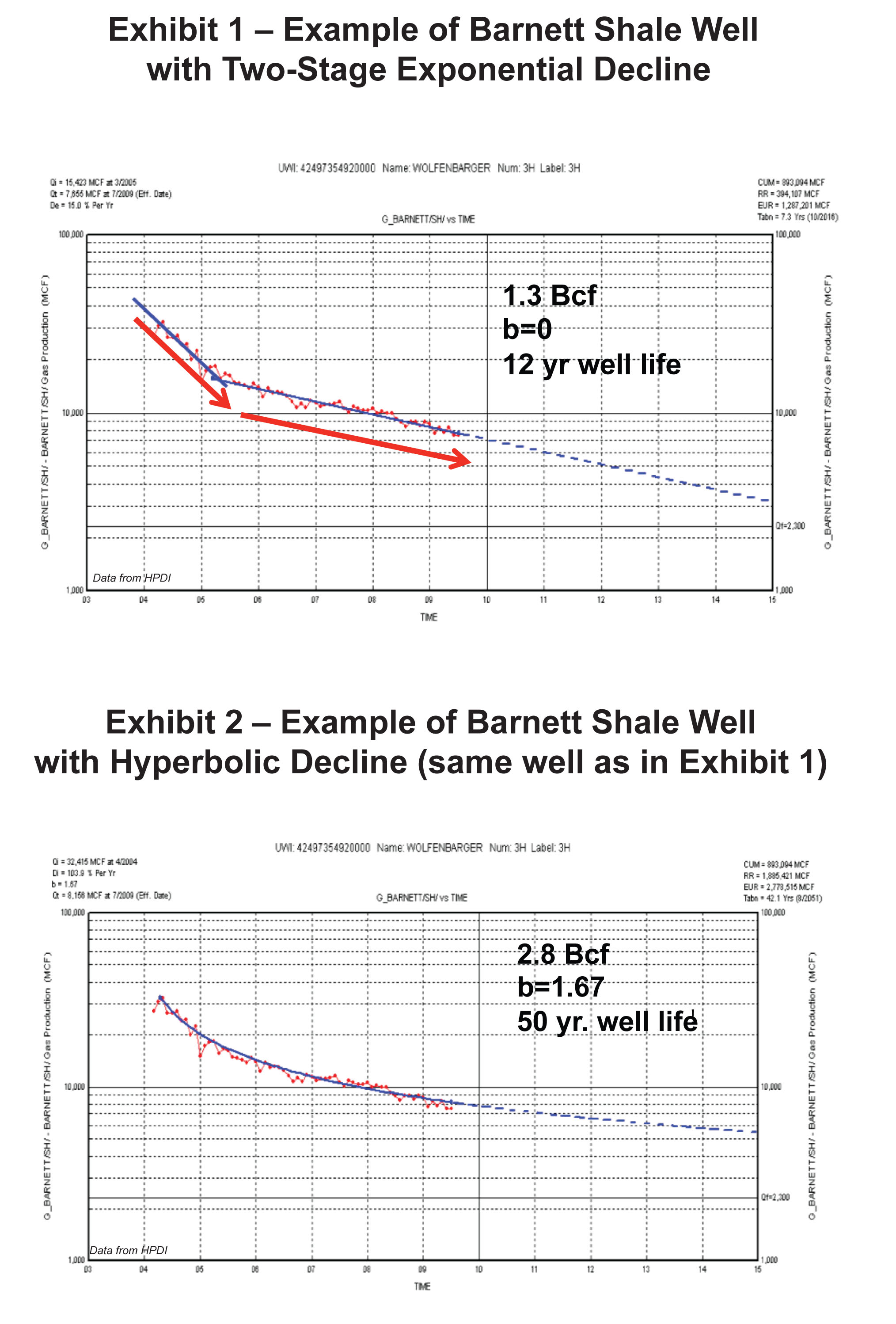
In contrast, most producers and industry analysts match the entire production history with a hyperbolic profile with resulting hyperbolic curvature, or “b”, exponents of more than 1.0 (Exhibit 2). This invariably results in a much higher EUR and longer well life because the decline rate progressively flattens beyond production history to very low terminal decline rates of a few percent.
We do not believe that it is appropriate to model the steep initial portion of the decline profile because it is not predictive of future behavior and is already accounted for in the cumulative production portion of the DCA (DCA is really about remaining reserves, after all).
Technical papers are mixed, but several peer-reviewed articles (see appendix) provide specific warnings against use of hyperbolic coefficients greater than 1.0, and specifically caution against including the initial steep transient decline rate in the matching process.
Aggregate production profiles for the Barnett, Fayetteville and Haynesville plays can be matched closely using the average well EUR presented in this study, providing an independent verification of these results. These points will be explained in more detail in subsequent sections including examples from different shale plays and operators.
Well Performance Evaluation Methodology
In this study, only horizontal wells were evaluated. With current technology and performance data, decline curve analysis (DCA) is the preferred technical approach to determine EUR for this analysis, supported by substantial empirical calibration from production histories for thousands of horizontal completions in the Barnett, Fayetteville and Haynesville shale plays. Other techniques such as volumetric calculations and reservoir simulation are limited by uncertainty and lack of calibration of recovery efficiency in the complex interaction between fracture stimulations, natural fractures and joints and shale matrix.
Investor presentations provided by operating companies typically show a group average composite curve normalized to the first month of production, combining well histories of varying duration. Our analysis indicates that this approach can be misleading, mainly because of survivorship bias (the increasing influence on the average over time by the survival of fewer and better performing wells) in the data but also by the inclusion of rate increases from re-stimulations that require additional capital investment. The older data points are representative of a much smaller sampling of wells.
We use a "vintaged grouping" method in our analyses to overcome much of the survivorship bias and effects of late-time well re-stimulations. First, we evaluate wells by operator because different operators have differing land positions that affect rock quality and well performance. Next, we vintage the wells by year of first production. This normalizes drilling and completion methods and permits recognition of performance improvement over time. Then we normalize wells within each vintaged group and do separate DCA for each group. Next, we use the number of wells that were active and the average EUR in each vintaged group to calculate a weighted average for each operator. Finally, we select a vintaged group with anomalously high EUR and conduct individual well DCA for all the wells in that group. We compare the average of the individual DCA with the the normalize group decline to calibrate our probable error for that operator. We do not adjust the weighted average EUR previously determined but this last technique gives us a measure of how much our DCA over-estimate EUR.
These points also will be explained in more detail in subsequent sections including examples from different shale plays and operators.
Barnett Well Performance
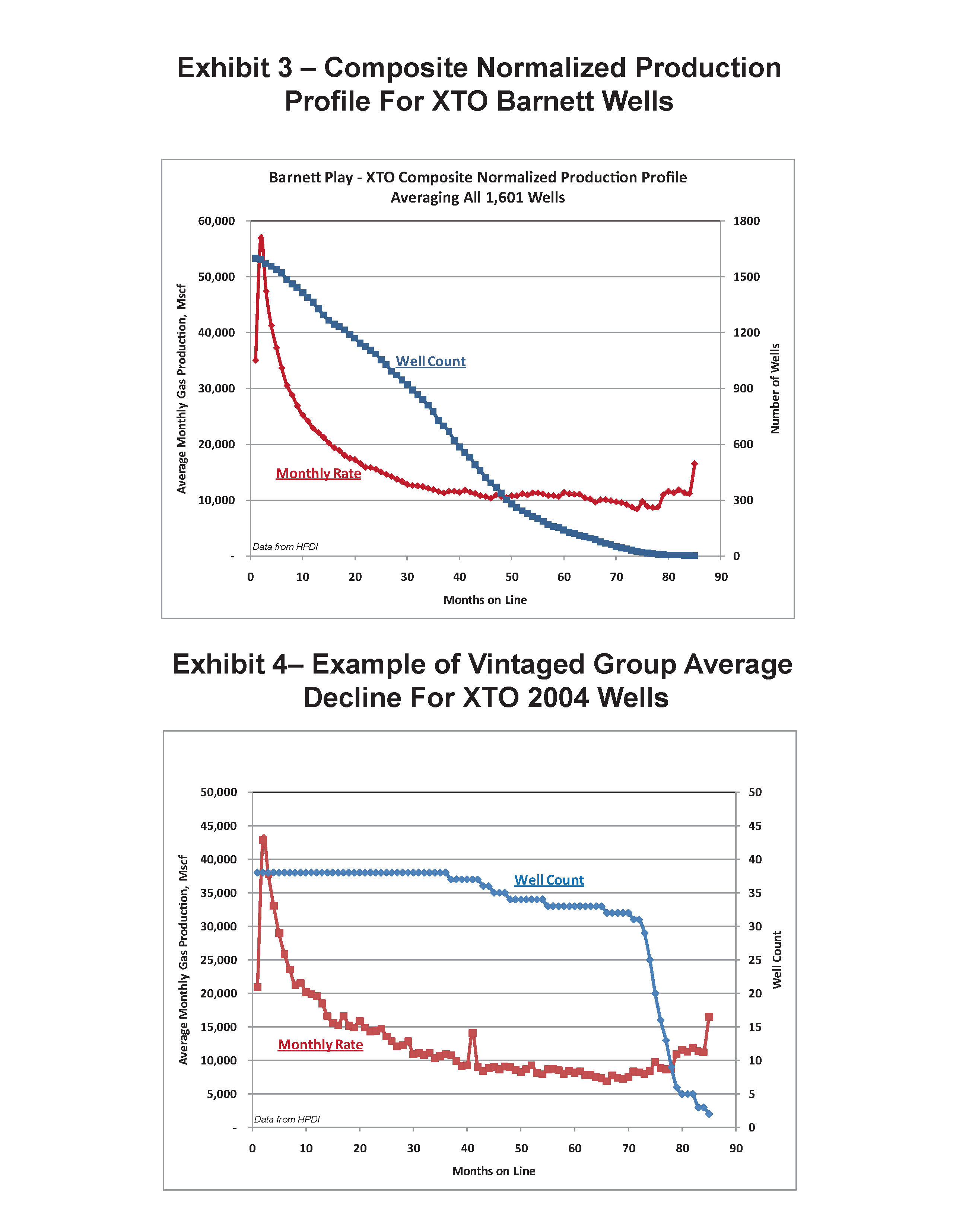
Exhibit 3 shows the group average production profile of 1,601 XTO wells in the Barnett Shale normalized to the first month of production. This example curve indicates virtually no decline for the last 4 years of production. The well count shows that the last year of the production decline trend is represented by less than 2% of the initial well count. The jump in average production after month 75 is the result of either survivorship bias (a few poorer wells drop out of the count resulting in an upward uplift because better wells survive) and/or re-stimulation.
Exhibit 4 features a subset of the wells in Exhibit 3 that is limited to wells with first production in 2004. Both Exhibits 3 and 4 show the effect of survivorship bias: as the number of wells decreases with time, the monthly rate flattens to a decline of almost zero because surviving high performance wells “lift” the average for later months. This flat decline profile is not seen in individual wells. This produces an artificially high EUR and long well life that is not real.
To test the accuracy of the vintaged group average approach, results were cross checked against the results of analyzing the individual decline trends for five different years and operators, summarized in Exhibit 5. This shows that DCA for individual wells is 21% to 48% lower. The average from individual well analysis will be more accurate than group averages (and therefore is considered the benchmark) because it eliminates survivorship bias and the distortion of the decline trend caused by stimulation work-overs (re-fracs).
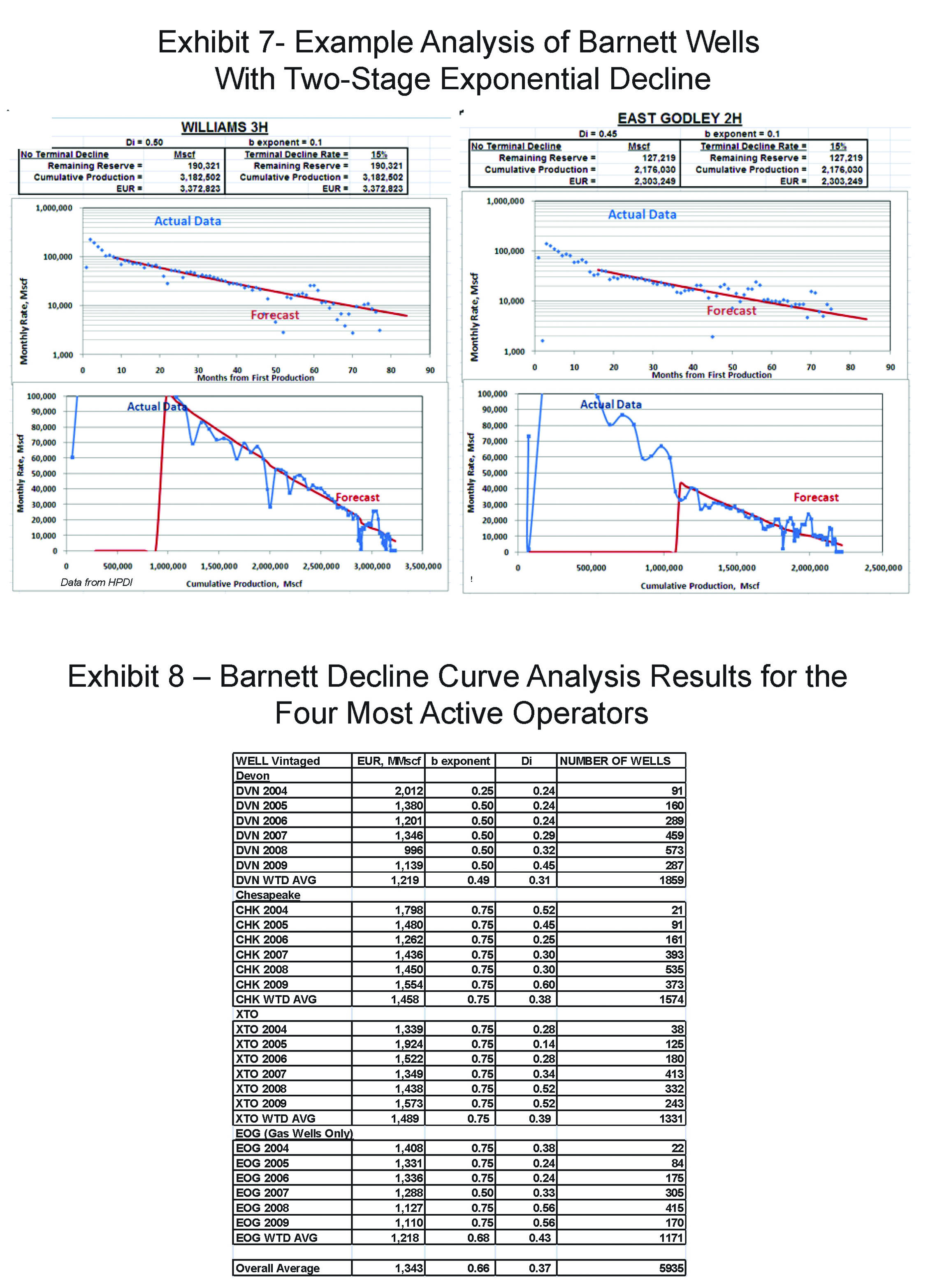
Exhibit 6 shows how we evaluate decline trends to determine remaining reserves, which are calculated from the extrapolation of the established decline trend until the well reaches its economic limit assumed to be 2,000 Mscf per month. One of the standard plots used in decline curve analysis is flow rate on a logarithmic scale plotted versus time as seen in Exhibit 7. This plot shows a typical example of individual decline behavior for a horizontal shale gas producer—a steep linear decline in the first 10-15 months followed by a second but flatter linear decline.
A straight line on this plot represents exponential decline with a constant decline rate, which typically indicates depletion of a boundary-dominated system or, in more technical petroleum engineering terms, pseudo-steady state flow. Exponential decline (coefficient b = 0) is a subset of hyperbolic decline. With a hyperbolic coefficient b > 0, the decline rate flattens, or decreases with time. This flattening can be observed in "infinite-acting" systems, or a system transitioning from the depletion of a near-wellbore high-permeability system to a lower permeability system with a larger pore volume. The flattening decline is caused by steadily increasing pore volume and drainage radius.
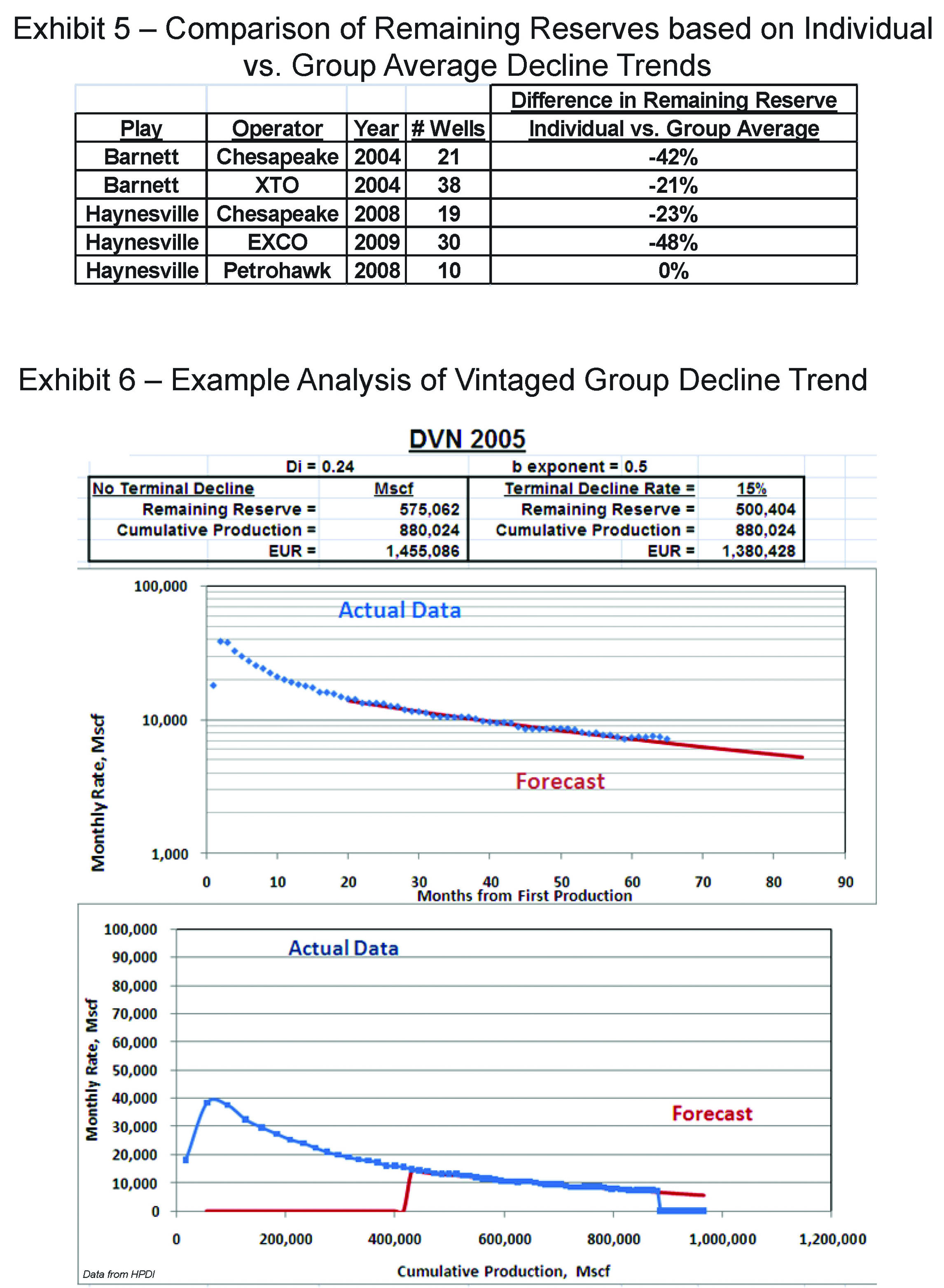
In Exhibit 7, please note the lower graphs showing monthly rate versus cumulative production, both on standard arithmetic scales. Exponential or boundary-dominated flows result in linear plots on this scale. This plot emphasizes deviations from exponential decay such as one would expect from hyperbolic decline. It also provides a useful reality check by putting into perspective the amount of remaining reserves being added to cumulative production used to calculate EUR.
Initial decline rates are steep but transition after 10-15 months to a flatter exponential decline trend that is the basis for extrapolating remaining reserves. This long period of flatter exponential decline represents depletion of a boundary-dominated system. Exhibit 8 summarizes EUR for the four principal producers in the Barnett Shale play based on our approach to DCA.
Fayetteville Well Performance
Based on our analysis of vintaged group curves that include 2,090 wells, the average EUR per well of the Fayetteville Shale play is 1.12 Bcf/well summarized in Exhibit 9. Southwestern- and BHP-operated wells (formerly Chesapeake) have the highest average at 1.2 Bcf/well, followed by XTO (formerly Petrohawk) at 0.8 Bcf/well. The decline trends were matched with moderate hyperbolic flattening (coefficient b=0.25 to 0.75), and initial decline rates, Di, averaging 72%/year, which is a steeper decline rate than observed in the Barnett Shale play.
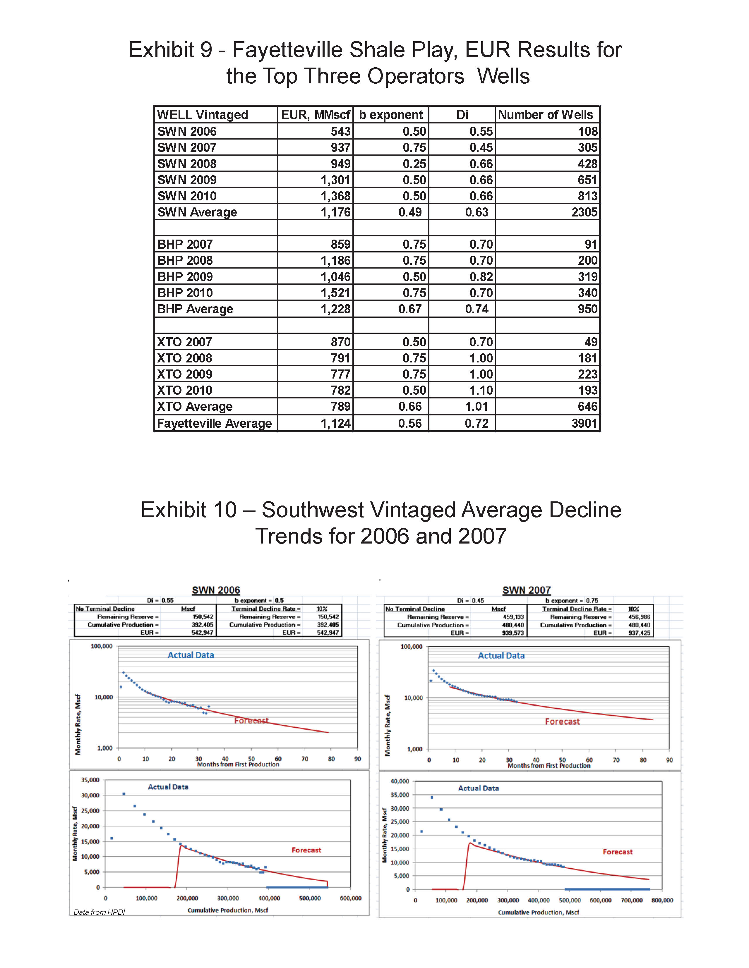
Exhibit 10 is an example of Southwestern Energy’s 2006 and 2007 wells (group average of 108 and 305 wells) following a similar two-stage exponential decline trend similar to most Barnett wells. The curve fit focuses on the established decline trend that begins after the first 12-months of steep decline, and ignores the scatter of the last few data points affected by survivorship bias.
In contrast to the Barnett Shale play, both Southwestern- and BHP-operated wells show substantial improvement in performance in both initial rates and EUR/well with time in the Fayetteville Shale play. For Southwestern, the maximum average monthly rate doubled from 2006 to 2008. The decline rates also appear to have increased, resulting in a proportionately smaller increase of 64% in EUR/well.
Haynesville Well Performance
The average EUR for Haynesville wells drilled by the four most active operators is 3.0 Bcf/well based on DCA trends from 263 wells. Petrohawk (now BHP) and EXCO results average 4.0 Bcf/well and are substantially better than Chesapeake and Encana results, which average 2.4 and 2.6 Bcf/well respectively. The better results achieved by Petrohawk and EXCO are probably because of their acreage positions in the core area of Desoto, Red River and Bossier parishes. Results are summarized in Exhibit 11. The vintaged average trends are matched with hyperbolic exponents ranging from 0.25 to 0.5, and initial decline rates, Di, averaging 1.4, the steepest decline of any of the shale gas plays evaluated.
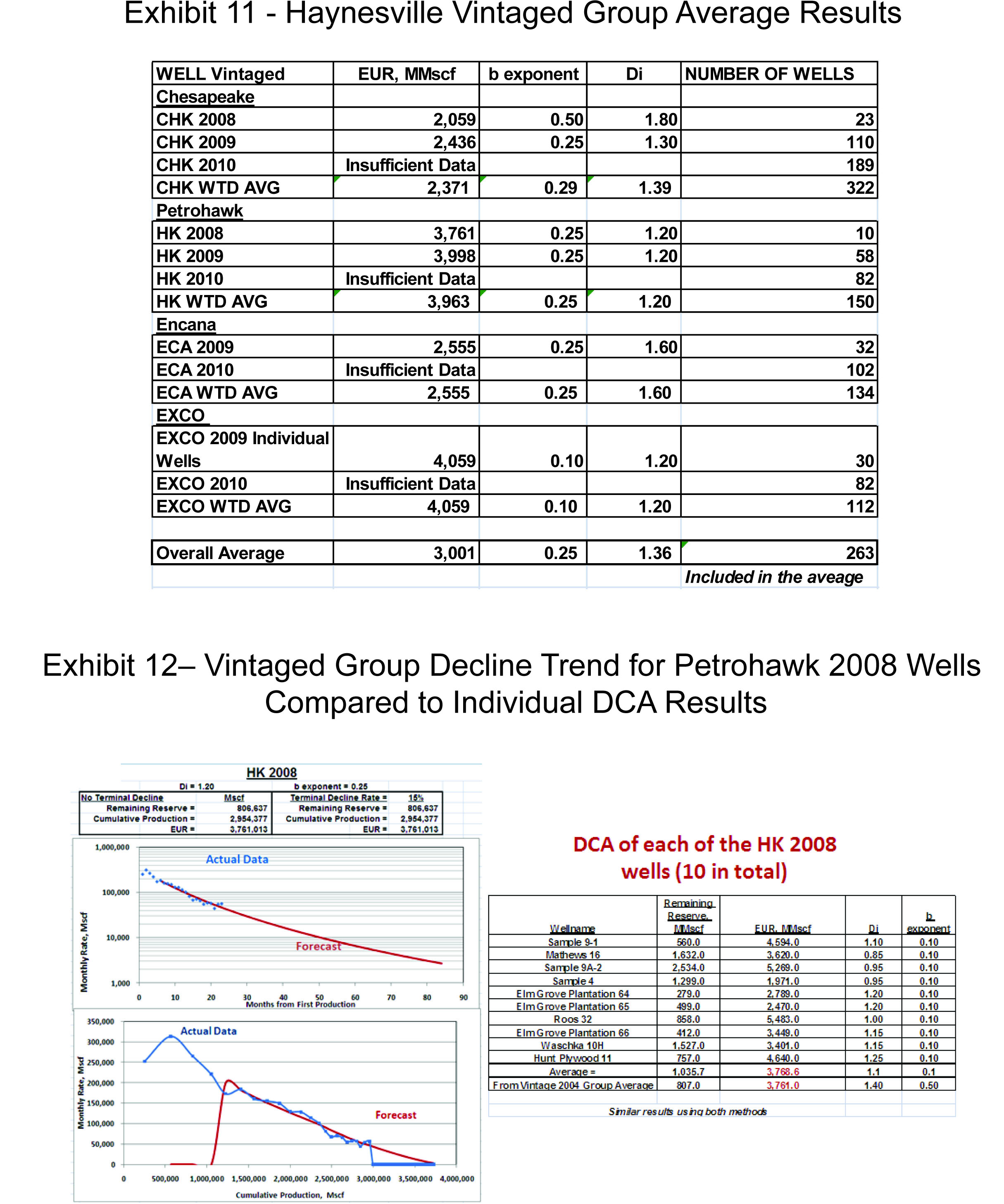
An example group average decline trend is shown in Exhibit 12 for Petrohawk wells with first production in 2008. This trend is based on 10 individual well decline trends, and the table included in Exhibit 10 shows the results of analyzing each individual decline. In this case, the result of extrapolating the average group decline provides similar results to the average from evaluating the decline of individual wells. The most important finding, however, from evaluating the decline of individual wells is that the decline trends appear to be more exponential than the group average, providing further evidence that the moderate hyperbolic flattening of the group average results from combining large numbers of wells with varied decline trends and durations.
Exhibit 13 shows two examples of exponential decline in individual Haynesville Shale wells. Unlike the two-stage declines of the Barnett and Fayetteville plays, these trends continue to follow the same exponential trends established in the early months of production. The rate versus cumulative production plots show that these wells are mostly depleted, and remaining reserves are a small portion of the EUR.
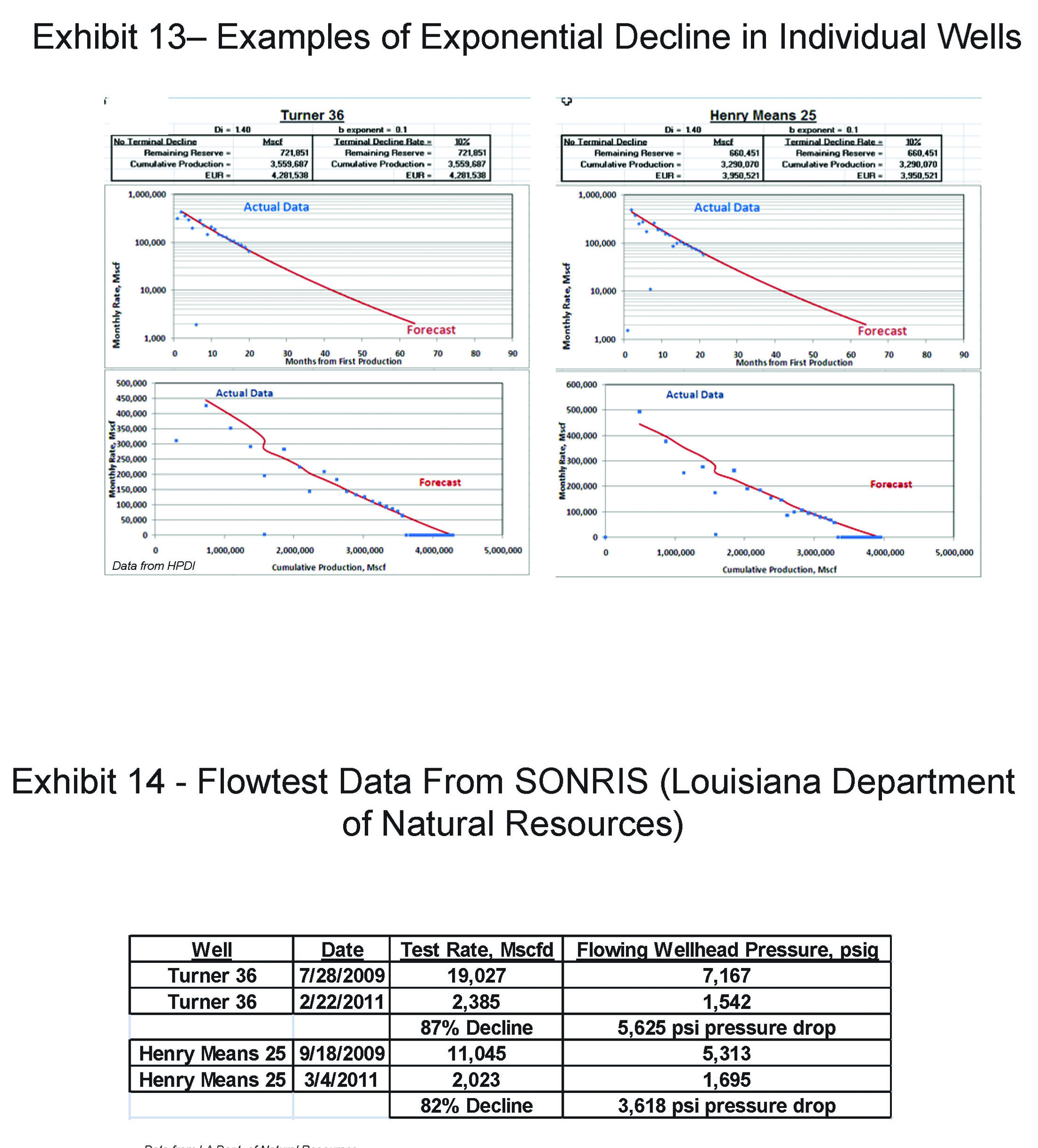
An implicit assumption in DCA is that flowing wellhead pressures are relatively stable. Significant increases in flowing wellhead pressure will cause the extrapolation of the rate decline trend to be too conservative and decreases will cause the extrapolation of the decline trend to be optimistic. Well test results for the two wells in Exhibit 13 are shown in Exhibit 14. Flowing wellhead pressures have declined by more than 3,500 psi in approximately 18 months as rates have declined by more than 80%.
Extrapolating the exponential decline of wells with such large decreases in wellhead pressures will result in an over-estimate of remaining reserves. Although a systematic study has not been attempted incorporating the flowing pressure data, examination of several dozen Haynesville wells indicates that the prevalent trend is for flowing wellhead pressures of Haynesville wells to decline by several thousand psi in the first 18 months of production as flow rates decrease and flowing wellhead pressures approach pipeline pressures.
The Haynesville play is unique among the shale gas plays because it is highly over-pressured, ranging from 0.75-0.85 psi/ft. This overpressure results in much higher initial rates than in other shale gas plays, some as high as 30 MMscfd. But, with pore pressures approaching the lithostatic gradient, pore pressures probably play a role in keeping fractures open, at least initially. As pressures deplete, the pore pressure can no longer counteract the lithostatic gradient, hence fracture permeability is probably reduced as the wells are depleted and fractures close, potentially explaining the much steeper decline rates observed in this trend.
Comparison to Operator Claims
Our analysis indicates that an average EUR/well is approximately one-half of the value typically claimed by major operators in the Barnett, Fayetteville, and Haynesville plays. Exhibit 15 provides a comparison for each of the plays. By focusing on the top four operators in each play, we evaluate the portfolio-level performance of the each play. By evaluating each operator’s wells by year of first production, we are able to recognize performance improvement.
A potential explanation for the difference between our EUR estimates and those of producers may be that they are describing the performance of the core area, whereas our approach includes all wells regardless of location operated by each of the top four most active companies.
A more important difference between results from this study and operator presentations is the long-term decline behavior of the wells. In multiple studies we have analyzed several thousands of individual wells in the Barnett, Fayetteville and Haynesville plays. Most wells are characterized by stable, exponential decline trends after the first year of steep decline, as previously shown in Exhibits 10 and 12. Additional individual well decline examples are available on request in presentation format for 118 Haynesville wells included in the individual vs. vintaged group average decline comparison shown in Exhibit 15.

Matching Aggregate Production Profiles for Shale Gas Plays
An important validation of the average EUR/well for a shale gas play is whether a type well with average properties can be used to model the overall production rate for that play. More specifically, the test is whether the well count and rate profile of the type well may be used to construct an aggregate field production profile that matches the actual data. The calculation of total rate for a play is based on the number of wells added through time and the calculated rate for various vintaged wells using a type well for the production rate. If the macro-level rate is comparable to the actual data, this test provides an independent validation of the type well.
For the Barnett Shale play, a two-stage model shown in Exhibit 16 provides a good match with the actual rate data assuming a 1.0 Bcf type well prior to January 2009, improving to 1.43 Bcf after January 2009. Exhibit 17 shows a good fit with Fayetteville aggregate production rates using improved well performance beginning in 2008 for the most active operator in the play, Southwestern Energy. The aggregate production profile for Haynesville wells in Louisiana can be matched closely with a 3.0 Bcf type well, the average observed EUR for the play as shown in Exhibit 18.

Economics
Discounted cash flow models were developed for each of the shale gas plays in this study to determine the break-even gas price. The EUR/well in each shale play is the most important assumption determining the breakeven gas price. Exhibits 19 and 20 show the breakeven gas prices for the average EUR/well values discussed in previous sections of this report. Assuming fully burdened costs including land acquisition, the breakeven gas price ranges from $8.31/MMBtu in the Fayetteville Shale to $8.75/MMBtu in the Barnett. With point-forward costs, which include only well drilling and completion costs and variable operating costs, the breakeven gas price is lower, ranging from $5.06/MMBtu in the Fayetteville to $6.80/MMBtu in the Haynesville.
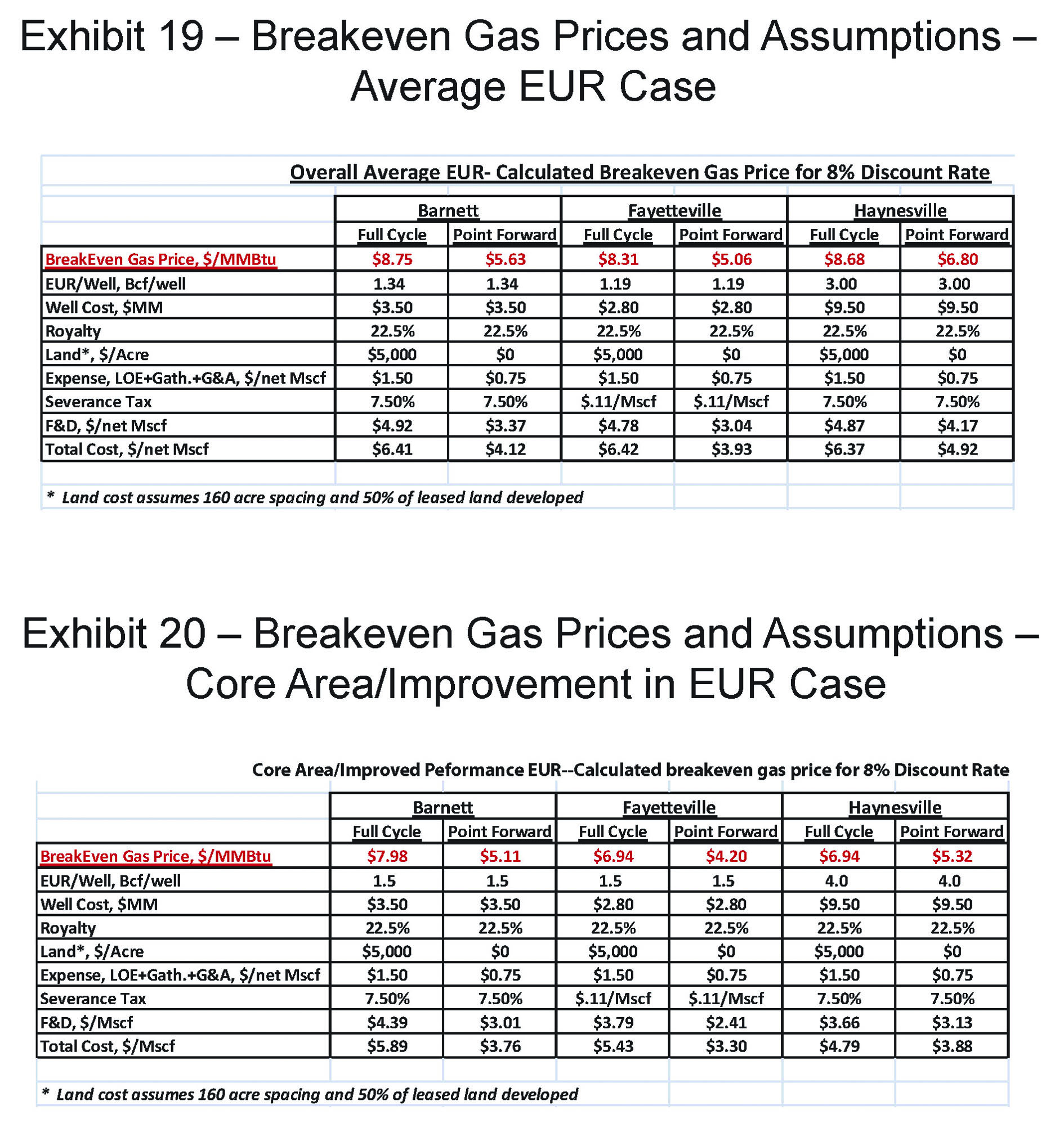
The fully-burdened case is intended to represent the long-term profitability of shale gas operators at the corporate level, including the highly competitive land acquisition phase. The point-forward case represents the price point where drilling additional wells returns the cost of capital, ignoring past costs and fixed costs such as general and administrative expenses.
Land costs vary considerably among operators, depending on whether the company was early or late in entering the play. Land costs are based on $5,000/acre leasing costs, which is high for an early entrance, but low for late entry, especially compared to recent purchases. Total land cost assumes that only one-half of the purchased acreage is eventually fully developed, accounting for aggressive land purchases prior to delineation of the relatively small core area. Assuming that only one-half of leased land is fully developed effectively doubles the land acquisition cost. Finally, well spacing is assumed to be 160 acres/well. Some operators claim final well spacing of 80 acres/well, but interference is likely to impact 5,000 ft lateral length wellbores at this spacing.
Operating costs are assumed to be $1.50/net Mscf based on a review of financial statements from several shale gas operators. This figure includes lease operating, workover, gathering, and general and administrative expenses. The variable component assumed in the point-forward basis is assumed to be $0.75/net Mscf. Royalty is assumed to be 22.5% in all cases, and severance taxes and ad valorem taxes are assumed to range from $0.11/Mscf in Arkansas to 7.5% in Texas and Louisiana.
The discount rate used for all break-even calculations is 8%/year, reflecting a relatively low cost of capital that may not be warranted for pure shale gas operators. A 10% discount rate would increase the breakeven price by $0.15-0.30/MMBtu.
Summary and Conclusions
We have shown that the true structural cost of shale gas production is higher than present prices can support ($4.15/mcf average price for the year ending July 30, 2011), and that per-well reserves are about one-half of the volumes claimed by operators. Relatively long-lived production history data in the Barnett and Fayetteville shale plays is compelling. A shorter production history for the Haynesville Shale play permits more latitude in forecasting projections. There is, however, sufficient data to conclude that results for the play are disappointing.
Our work on the three most mature shale plays has profound implications. Facts indicate that most wells are not commercial at current gas prices and require prices at least in the range of $8.00 to $9.00/mcf to break even on full-cycle prices, and $5.00 to $6.00/mcf on point-forward prices. Our price forecasts ($4.00-4.55/mcf average through 2012) are below $8.00/mcf for the next 18 months. It is, therefore, possible that some producers will be unable to maintain present drilling levels from cash flow, joint ventures, asset sales and stock offerings.
Decline rates indicate that a decrease in drilling by any of the major producers in the shale gas plays would reveal the insecurity of supply. This is especially true in the case of the Haynesville Shale play where initial rates are about three times higher than in the Barnett or Fayetteville. Already, rig rates are dropping in the Haynesville as operators shift emphasis to more liquid-prone objectives that have even lower gas rates. This might create doubt about the paradigm of cheap and abundant shale gas supply and have a cascading effect on confidence and capital availability.
On the other hand, major oil companies, foreign investors and overseas energy companies have shown a surprising appetite for joint ventures and acquisitions of producers in these plays. Although this trend might result in a different cast of players, it may also introduce a stabilizing effect on the distress scenario described in the previous paragraph. The entry of better-capitalized producers does not change the economic fundamentals of shale gas, but it suggests that there may be strategic reasons for large companies to pursue market share in the North American gas arena.
We suspect that the current euphoria about shale gas will follow the path of other energy panaceas including coal-bed methane and tight sandstone gas. Shale gas will remain an important part of the North American energy landscape but its costs will almost certainly be higher, and its abundance less than many now believe. Producer behavior will be modified by the effect of changing perceptions on capital availability and the entry of new, more substantial players.
APPENDIX
Suggested references:
Cheng, Y. et al, 2005. Practical Applications of Probabilistic Approach to Estimate Reserves Using Production Decline Data. Paper SPE 95974 presented at 2005 SPE Annual Technical Conference, Dallas, TX, 9-12 October 2005.
Fan, L, et al, 2011. The Bottom Line of Horizontal Well Production Decline in the Barnett Formation. Paper SPE 141263 presented at the SPE Production and Operations Symposium in Oklahoma City, OK 27-29 March, 2011.
Fetkovitch, M. J. et al, 1990. Depletion Performance of Layered Reservoirs Without Crossflow. Paper SPE 18266 published in SPE Formation Evaluation, September 1990.
Ilk, D, et al, 2008. Exponential vs. Hyperbolic Decline in Tight Gas Sands – Understanding the Origins and Implications for Reserve Estimates Using Arp’s Decline Curves. Paper SPE 116731 presented at SPE Annual Technical Conference, Denver, CO, 21-24 September 2008.
Lee, W. J. et al, 2010. Gas Reserves Estimating in Resource Plays. Paper SPE 130102 presented at the SPE Unconventional Gas Conference in Pittsburg, PA 23-25 February 2010.
Mattar, L. et al, 2008. Production Analysis and Forecasting of Shale Gas Reservoirs: Case History-Basd Approach. Paper SPE 119897 presented at the Shale Gas Production Conference, Fort Worth, TX, 16-18 November 2008.
Vanorsdale, C. R., 1987. Evaluation of Devonian Shale Gas Reservoirs. Paper SPE 14446 published in SPE Reservoir Engineering, May 1987.